Tutorial with Synthetic Data

This is an example notebook with overview of the usage of the modules in tscluster.

!pip install -r https://raw.githubusercontent.com/tscluster-project/tscluster/main/requirements.txt
!pip install tscluster # install tscluster

Requirement already satisfied: numpy>=1.26 in /usr/local/lib/python3.10/dist-packages (from -r https://raw.githubusercontent.com/tscluster-project/tscluster/main/requirements.txt (line 1)) (1.26.4)
Requirement already satisfied: pandas>=2.2 in /usr/local/lib/python3.10/dist-packages (from -r https://raw.githubusercontent.com/tscluster-project/tscluster/main/requirements.txt (line 2)) (2.2.2)
Requirement already satisfied: matplotlib<3.9,>=3.8 in /usr/local/lib/python3.10/dist-packages (from -r https://raw.githubusercontent.com/tscluster-project/tscluster/main/requirements.txt (line 3)) (3.8.4)
Requirement already satisfied: python-dateutil>=2.8.2 in /usr/local/lib/python3.10/dist-packages (from pandas>=2.2->-r https://raw.githubusercontent.com/tscluster-project/tscluster/main/requirements.txt (line 2)) (2.8.2)
Requirement already satisfied: pytz>=2020.1 in /usr/local/lib/python3.10/dist-packages (from pandas>=2.2->-r https://raw.githubusercontent.com/tscluster-project/tscluster/main/requirements.txt (line 2)) (2023.4)
Requirement already satisfied: tzdata>=2022.7 in /usr/local/lib/python3.10/dist-packages (from pandas>=2.2->-r https://raw.githubusercontent.com/tscluster-project/tscluster/main/requirements.txt (line 2)) (2024.1)
Requirement already satisfied: contourpy>=1.0.1 in /usr/local/lib/python3.10/dist-packages (from matplotlib<3.9,>=3.8->-r https://raw.githubusercontent.com/tscluster-project/tscluster/main/requirements.txt (line 3)) (1.2.1)
Requirement already satisfied: cycler>=0.10 in /usr/local/lib/python3.10/dist-packages (from matplotlib<3.9,>=3.8->-r https://raw.githubusercontent.com/tscluster-project/tscluster/main/requirements.txt (line 3)) (0.12.1)
Requirement already satisfied: fonttools>=4.22.0 in /usr/local/lib/python3.10/dist-packages (from matplotlib<3.9,>=3.8->-r https://raw.githubusercontent.com/tscluster-project/tscluster/main/requirements.txt (line 3)) (4.51.0)
Requirement already satisfied: kiwisolver>=1.3.1 in /usr/local/lib/python3.10/dist-packages (from matplotlib<3.9,>=3.8->-r https://raw.githubusercontent.com/tscluster-project/tscluster/main/requirements.txt (line 3)) (1.4.5)
Requirement already satisfied: packaging>=20.0 in /usr/local/lib/python3.10/dist-packages (from matplotlib<3.9,>=3.8->-r https://raw.githubusercontent.com/tscluster-project/tscluster/main/requirements.txt (line 3)) (24.0)
Requirement already satisfied: pillow>=8 in /usr/local/lib/python3.10/dist-packages (from matplotlib<3.9,>=3.8->-r https://raw.githubusercontent.com/tscluster-project/tscluster/main/requirements.txt (line 3)) (9.4.0)
Requirement already satisfied: pyparsing>=2.3.1 in /usr/local/lib/python3.10/dist-packages (from matplotlib<3.9,>=3.8->-r https://raw.githubusercontent.com/tscluster-project/tscluster/main/requirements.txt (line 3)) (3.1.2)
Requirement already satisfied: six>=1.5 in /usr/local/lib/python3.10/dist-packages (from python-dateutil>=2.8.2->pandas>=2.2->-r https://raw.githubusercontent.com/tscluster-project/tscluster/main/requirements.txt (line 2)) (1.16.0)
Requirement already satisfied: tscluster in /usr/local/lib/python3.10/dist-packages (1.0.4)
Requirement already satisfied: numpy>=1.26 in /usr/local/lib/python3.10/dist-packages (from tscluster) (1.26.4)
Requirement already satisfied: scipy>=1.10 in /usr/local/lib/python3.10/dist-packages (from tscluster) (1.11.4)
Requirement already satisfied: gurobipy>=11.0 in /usr/local/lib/python3.10/dist-packages (from tscluster) (11.0.2)
Requirement already satisfied: tslearn>=0.6.3 in /usr/local/lib/python3.10/dist-packages (from tscluster) (0.6.3)
Requirement already satisfied: h5py>=3.10 in /usr/local/lib/python3.10/dist-packages (from tscluster) (3.11.0)
Requirement already satisfied: pandas>=2.2 in /usr/local/lib/python3.10/dist-packages (from tscluster) (2.2.2)
Requirement already satisfied: matplotlib<3.9,>=3.8 in /usr/local/lib/python3.10/dist-packages (from tscluster) (3.8.4)
Requirement already satisfied: contourpy>=1.0.1 in /usr/local/lib/python3.10/dist-packages (from matplotlib<3.9,>=3.8->tscluster) (1.2.1)
Requirement already satisfied: cycler>=0.10 in /usr/local/lib/python3.10/dist-packages (from matplotlib<3.9,>=3.8->tscluster) (0.12.1)
Requirement already satisfied: fonttools>=4.22.0 in /usr/local/lib/python3.10/dist-packages (from matplotlib<3.9,>=3.8->tscluster) (4.51.0)
Requirement already satisfied: kiwisolver>=1.3.1 in /usr/local/lib/python3.10/dist-packages (from matplotlib<3.9,>=3.8->tscluster) (1.4.5)
Requirement already satisfied: packaging>=20.0 in /usr/local/lib/python3.10/dist-packages (from matplotlib<3.9,>=3.8->tscluster) (24.0)
Requirement already satisfied: pillow>=8 in /usr/local/lib/python3.10/dist-packages (from matplotlib<3.9,>=3.8->tscluster) (9.4.0)
Requirement already satisfied: pyparsing>=2.3.1 in /usr/local/lib/python3.10/dist-packages (from matplotlib<3.9,>=3.8->tscluster) (3.1.2)
Requirement already satisfied: python-dateutil>=2.7 in /usr/local/lib/python3.10/dist-packages (from matplotlib<3.9,>=3.8->tscluster) (2.8.2)
Requirement already satisfied: pytz>=2020.1 in /usr/local/lib/python3.10/dist-packages (from pandas>=2.2->tscluster) (2023.4)
Requirement already satisfied: tzdata>=2022.7 in /usr/local/lib/python3.10/dist-packages (from pandas>=2.2->tscluster) (2024.1)
Requirement already satisfied: scikit-learn in /usr/local/lib/python3.10/dist-packages (from tslearn>=0.6.3->tscluster) (1.2.2)
Requirement already satisfied: numba in /usr/local/lib/python3.10/dist-packages (from tslearn>=0.6.3->tscluster) (0.58.1)
Requirement already satisfied: joblib in /usr/local/lib/python3.10/dist-packages (from tslearn>=0.6.3->tscluster) (1.4.2)
Requirement already satisfied: six>=1.5 in /usr/local/lib/python3.10/dist-packages (from python-dateutil>=2.7->matplotlib<3.9,>=3.8->tscluster) (1.16.0)
Requirement already satisfied: llvmlite<0.42,>=0.41.0dev0 in /usr/local/lib/python3.10/dist-packages (from numba->tslearn>=0.6.3->tscluster) (0.41.1)
Requirement already satisfied: threadpoolctl>=2.0.0 in /usr/local/lib/python3.10/dist-packages (from scikit-learn->tslearn>=0.6.3->tscluster) (3.5.0)

Importing Libraries

# uncomment the line below if widget is enable in your environment. This is useful for making tsplot's waterfall_plot interactive
# %matplotlib widget

import os

import numpy as np
import pandas as pd
import requests

from tscluster.opttscluster import OptTSCluster
from tscluster.tskmeans import TSKmeans, TSGlobalKmeans
from tscluster.preprocessing import TSStandardScaler, TSMinMaxScaler
from tscluster.preprocessing.utils import load_data, tnf_to_ntf, ntf_to_tnf, to_dfs, broadcast_data
from tscluster.metrics import inertia, max_dist
from tscluster.tsplot import tsplot

par_dir = "tscluster_sample_data"

# download the sample data

# we need to store the data on the local Colab file system
!wget https://raw.githubusercontent.com/tscluster-project/tscluster/main/test/tscluster_sample_data.zip

if not os.path.exists(par_dir):
        os.makedirs(par_dir)

# unzipping the downloaded file to 'tscluster_sample_data' directory in local file system
!unzip -o tscluster_sample_data.zip -d tscluster_sample_data

--2024-05-22 00:02:47--  https://raw.githubusercontent.com/tscluster-project/tscluster/main/test/tscluster_sample_data.zip
Resolving raw.githubusercontent.com (raw.githubusercontent.com)... 185.199.108.133, 185.199.109.133, 185.199.110.133, ...
Connecting to raw.githubusercontent.com (raw.githubusercontent.com)|185.199.108.133|:443... connected.
HTTP request sent, awaiting response... 200 OK
Length: 11197 (11K) [application/zip]
Saving to: ‘tscluster_sample_data.zip.2’


      tscluster   0%[                    ]       0  --.-KB/s

tscluster_sample_da 100%[===================>] 10.93K –.-KB/s in 0s

2024-05-22 00:02:47 (34.9 MB/s) - ‘tscluster_sample_data.zip.2’ saved [11197/11197]

Archive: tscluster_sample_data.zip
inflating: tscluster_sample_data/synthetic_csv/timestep_0.csv inflating: tscluster_sample_data/synthetic_csv/timestep_1.csv inflating: tscluster_sample_data/synthetic_csv/timestep_2.csv inflating: tscluster_sample_data/synthetic_csv/timestep_3.csv inflating: tscluster_sample_data/synthetic_csv/timestep_4.csv inflating: tscluster_sample_data/synthetic_csv2/year-2000.csv inflating: tscluster_sample_data/synthetic_csv2/year-2005.csv inflating: tscluster_sample_data/synthetic_csv2/year-2010.csv inflating: tscluster_sample_data/synthetic_csv2/year-2015.csv inflating: tscluster_sample_data/synthetic_csv2/year-2020.csv inflating: tscluster_sample_data/synthetic_json/timestep_0.json inflating: tscluster_sample_data/synthetic_json/timestep_1.json inflating: tscluster_sample_data/synthetic_json/timestep_2.json inflating: tscluster_sample_data/synthetic_json/timestep_3.json inflating: tscluster_sample_data/synthetic_json/timestep_4.json inflating: tscluster_sample_data/synthetic_npy/timestep_0.npy inflating: tscluster_sample_data/synthetic_npy/timestep_1.npy inflating: tscluster_sample_data/synthetic_npy/timestep_2.npy inflating: tscluster_sample_data/synthetic_npy/timestep_3.npy inflating: tscluster_sample_data/synthetic_npy/timestep_4.npy inflating: tscluster_sample_data/sythetic_data.npy

os.chdir(par_dir)

Loading Data

from a npy file

If data is a numpy array stored as a .npy file, you can use the load_data function to load it.

X, label_dict = load_data("./sythetic_data.npy")
X.shape

(10, 15, 1)

The load_data function returns a tuple, the first value of the tuple is the loaded data (a 3-D array in ‘TNF’ format), while the second value of the tuple is the label_dict of the data. The label_dict is a dictionary whose keys are ‘T’, ‘N’, and ‘F’ (which are the number of time steps, entities, and features respectively). Value of each key is a list such that the value of key: - ‘T’ is a list of names/labels of each time step to be used as index of each dataframe. If None, range(0, T) is used. Where T is the number of time steps in the fitted data - ‘N’ (ignored) is a list of names/labels of each entity. If None, range(0, N) is used. Where N is the number of entities/observations in the fitted data - ‘F’ is a list of names/labels of each feature to be used as column of each dataframe. If None, range(0, F) is used. Where F is the number of features in the fitted data

# checking the label_dict
print(label_dict)

{'T': [0, 1, 2, 3, 4, 5, 6, 7, 8, 9], 'N': [0, 1, 2, 3, 4, 5, 6, 7, 8, 9, 10, 11, 12, 13, 14], 'F': [0]}

As seen in the output above, the data has 10 time steps, 15 entities and 1 feature. The data is a synthetic data created for demonstration purposes in this notebook. The time steps could be years e.g. year 2001 to 2010, the entities could be zipcodes/postal codes e.g 15 postal codes in Toronto, and the features could be any variable(s) measured for each entity in each time step e.g. population.

This notebook will focus on using the common attributes and methods of the modules available in tscluster. For an example notebook with applications to real-life data, see this notebook.

Checking the first time steps of the first five entities.

X[:5, :5, :]

array([[[15.09011416],
        [15.09011416],
        [ 6.92001802],
        [ 6.92001802],
        [11.39918324]],

       [[10.4044138 ],
        [10.4044138 ],
        [ 8.76582237],
        [ 8.76582237],
        [11.33740921]],

       [[ 8.67698496],
        [ 8.67698496],
        [ 9.55393712],
        [ 9.55393712],
        [10.57717395]],

       [[ 6.01642654],
        [ 6.01642654],
        [10.63908781],
        [10.63908781],
        [10.6098427 ]],

       [[ 4.89052455],
        [ 4.89052455],
        [11.61399362],
        [11.61399362],
        [ 9.34167455]]])

from a list

Data can also be loaded from a list. This can be a list of 2-D numpy arrays, or list of pandas dataframes, or list of file paths. By default, the list is of length T (number of time steps), where each element of the list is interpreted as a data for all entities at a particular time step. Set the arr_format parameter to ‘NTF’ to specify that each element of the input list is the time series data for a particular entity for all time steps. Valid files are .npy, .npz, .json, xlsx, .csv or any file readable by pandas.read_csv function.

Reading from a list of dataframes

df1 = pd.DataFrame({
    'f1': np.arange(5),
    'f2': np.arange(5, 10)
}, index=['e'+str(i+1) for i in range(5)]
                  )
df1

	f1	f2
e1	0	5
e2	1	6
e3	2	7
e4	3	8
e5	4	9

df2 = pd.DataFrame({
    'f2': np.arange(105, 110),
    'f1': np.arange(100, 105)
}, index=['e'+str(i+1) for i in range(5)]
                  )
df2

	f2	f1
e1	105	100
e2	106	101
e3	107	102
e4	108	103
e5	109	104

X_arr, label_dict = load_data([df1, df2])
print(f"shape of X_arr is {X_arr.shape}")
X_arr = X_arr.astype(np.float64)
X_arr

shape of X_arr is (2, 5, 2)

array([[[  0.,   5.],
        [  1.,   6.],
        [  2.,   7.],
        [  3.,   8.],
        [  4.,   9.]],

       [[100., 105.],
        [101., 106.],
        [102., 107.],
        [103., 108.],
        [104., 109.]]])

label_dict

{'T': [0, 1], 'N': ['e1', 'e2', 'e3', 'e4', 'e5'], 'F': ['f1', 'f2']}

To get the output in ‘NTF’ format, set the output_arr_format parameter to ‘NTF’

X_arr, label_dict = load_data([df1, df2], output_arr_format='NTF')
print(f"shape of X_arr is {X_arr.shape}")
X_arr

shape of X_arr is (5, 2, 2)

array([[[  0.,   5.],
        [100., 105.]],

       [[  1.,   6.],
        [101., 106.]],

       [[  2.,   7.],
        [102., 107.]],

       [[  3.,   8.],
        [103., 108.]],

       [[  4.,   9.],
        [104., 109.]]])

label_dict # label_dict will remain the same

{'T': [0, 1], 'N': ['e1', 'e2', 'e3', 'e4', 'e5'], 'F': ['f1', 'f2']}

The same applies to list of file paths. E.g.

file_list = [
    "./synthetic_csv/timestep_0.csv",
    "./synthetic_csv/timestep_1.csv",
    "./synthetic_csv/timestep_2.csv",
    "./synthetic_csv/timestep_3.csv",
    "./synthetic_csv/timestep_4.csv"
]

X_arr, label_dict = load_data(file_list)
print(f"shape of X_arr is {X_arr.shape}")

shape of X_arr is (5, 20, 2)

label_dict

{'T': [0, 1, 2, 3, 4],
 'N': [0, 1, 2, 3, 4, 5, 6, 7, 8, 9, 10, 11, 12, 13, 14, 15, 16, 17, 18, 19],
 'F': [0, 1]}

You can also pass arguments to the file reader used by using the read_file_args parameter. This parameter accepts a dictionary where the keys are the names of the file reader parameters (in string), and the values are the values of the file reader parameter. E.g. if file reader is pd.read_csv (reader for csv file), you can pass names and skiprows arguments (and basically any argument you want to pass to the file reader).

file_list = [
    "./synthetic_csv/timestep_0.csv",
    "./synthetic_csv/timestep_1.csv",
    "./synthetic_csv/timestep_2.csv",
    "./synthetic_csv/timestep_3.csv",
    "./synthetic_csv/timestep_4.csv"
]

X_arr, label_dict = load_data(file_list, read_file_args={'names': ['x1', 'x2'], 'skiprows': 10})
print(f"shape of X_arr is {X_arr.shape}")

shape of X_arr is (5, 10, 2)

label_dict

{'T': [0, 1, 2, 3, 4], 'N': [0, 1, 2, 3, 4, 5, 6, 7, 8, 9], 'F': ['x1', 'x2']}

from a directory

You can instead pass a directory path (as a string) to the load_data function. In this case, the suffix (not file extension) of the filenames will be used for ordering the files before loading them as different timesteps. The suffix consists of characters after suffix_sep (not including file extension). The default value for suffix_sep is an undescore “_“. E.g. if the ‘synthetic_csv’ directory contains the following files:

timestep_1.csv
timestep_2.csv
timestep_3.csv
timestep_4.csv

We can read the files as follows:

X_arr, label_dict = load_data('./synthetic_csv')
print(f"shape of X_arr is {X_arr.shape}")

shape of X_arr is (5, 20, 2)

label_dict

{'T': [0, 1, 2, 3, 4],
 'N': [0, 1, 2, 3, 4, 5, 6, 7, 8, 9, 10, 11, 12, 13, 14, 15, 16, 17, 18, 19],
 'F': [0, 1]}

The suffixes of the filenames may not neccessarily start from 1 or have an interval of 1. For example, the filenames could be:

year-2000.csv
year-2005.csv
year-2010.csv
year-2015.csv
year-2020.csv

So long the suffixes can be sorted and there is a consistent suffix separator (“-” is this case), the directory can be parsed by load_data function.

# checking how the head of a single
pd.read_csv('./synthetic_csv2/year-2005.csv').head()

	Unnamed: 0	x1	x2	x3
0	i1	1.144403	1.384766	-0.296697
1	i2	-0.221455	-2.379010	1.616871
2	i3	1.533177	-1.650524	-0.548531
3	i4	-0.615204	0.794567	-0.726242
4	i5	0.622818	-0.129735	-0.723215

# if we were to indicate to pandas that the first column is the index and the first row is the header, we would have done
pd.read_csv('./synthetic_csv2/year-2005.csv', index_col=[0], header=0).head()

	x1	x2	x3
i1	1.144403	1.384766	-0.296697
i2	-0.221455	-2.379010	1.616871
i3	1.533177	-1.650524	-0.548531
i4	-0.615204	0.794567	-0.726242
i5	0.622818	-0.129735	-0.723215

# using load_data function
X_arr, label_dict = load_data('./synthetic_csv2',
                              suffix_sep='-',
                              use_suffix_as_label=True,
                              read_file_args={'index_col': [0], 'header': 0})
print(f"shape of X_arr is {X_arr.shape}")

shape of X_arr is (5, 10, 3)

print(label_dict)

{'T': ['2000', '2005', '2010', '2015', '2020'], 'N': ['i1', 'i10', 'i2', 'i3', 'i4', 'i5', 'i6', 'i7', 'i8', 'i9'], 'F': ['x1', 'x2', 'x3']}

Data Conversion

to_dfs

We can convert a 3-D array to a list of dataframes using the to_dfs function. This is basically the reverse process of load_dict in that it takes a 3-D array and an optional label_dict, and returns a list of dataframes. Similar to load_dict function, you can use arr_format and output_df_format to specify the format of the input data and output data respectively.

dfs = to_dfs(X_arr, label_dict)
print(f"Length of dfs is: {len(dfs)}")
dfs[0].head() # first five rows of the first dataframe in the list

Length of dfs is: 5

	x1	x2	x3
i1	0.496714	-0.138264	-0.291524
i10	0.097078	0.968645	0.626228
i2	-0.463418	-0.465730	-0.312976
i3	1.465649	-0.225776	0.488591
i4	-0.601707	1.852278	-0.078235

tnf_to_ntf

tnf_to_ntf function can be used to convert a data from ‘TNF’ format to ‘NTF’ format. E.g

print(f"Shape of X_arr in 'TNF' format is: {X_arr.shape}")

X_arr_ntf = tnf_to_ntf(X_arr)

print(f"Shape of X_arr in 'NTF' format is: {X_arr_ntf.shape}")

Shape of X_arr in 'TNF' format is: (5, 10, 3)
Shape of X_arr in 'NTF' format is: (10, 5, 3)

ntf_to_tnf

Similarly, ntf_to_tnf function can be used to convert from ‘NTF’ format to ‘TNF’ format. E.g.

print(f"Shape of X_arr in 'NTF' format is: {X_arr_ntf.shape}")

print(f"Shape of X_arr in 'TNF' format is: {ntf_to_tnf(X_arr_ntf).shape}")

Shape of X_arr in 'NTF' format is: (10, 5, 3)
Shape of X_arr in 'TNF' format is: (5, 10, 3)

broadcast_data

If you want to broadcast a fixed cluster center along the time axis, you can use broadcast_data function. E.g. if you have fixed cluster centers as a 2-D array of shape (K, F), where K is the number of clusters and F is the number of features; you can convert it to a 3-D array such that the first axis is the time axis. This is usefule especially when dealing with fixed center or fixed assignment because they return (for memory efficiency) a 2-D array and a 1-D array respectively.

np.random.seed(0)
cluster_centers = np.random.randn(3, 2)
cluster_centers

array([[ 1.76405235,  0.40015721],
       [ 0.97873798,  2.2408932 ],
       [ 1.86755799, -0.97727788]])

T = 3 # number of time steps
cluster_centers_broadcasted, _ = broadcast_data(T, cluster_centers=cluster_centers)
cluster_centers_broadcasted

array([[[ 1.76405235,  0.40015721],
        [ 0.97873798,  2.2408932 ],
        [ 1.86755799, -0.97727788]],

       [[ 1.76405235,  0.40015721],
        [ 0.97873798,  2.2408932 ],
        [ 1.86755799, -0.97727788]],

       [[ 1.76405235,  0.40015721],
        [ 0.97873798,  2.2408932 ],
        [ 1.86755799, -0.97727788]]])

You can also broadcast labels. E.g if the cluster labels is a 1-D numpy array of shape (N, ).

np.random.seed(2)
labels = np.random.choice([0, 1, 2], 10)
labels

array([0, 1, 0, 2, 2, 0, 2, 1, 1, 2])

T = 3 # number of time steps
_, labels_broadcasted = broadcast_data(T, labels=labels)
labels_broadcasted

array([[0, 0, 0],
       [1, 1, 1],
       [0, 0, 0],
       [2, 2, 2],
       [2, 2, 2],
       [0, 0, 0],
       [2, 2, 2],
       [1, 1, 1],
       [1, 1, 1],
       [2, 2, 2]])

You can also broadcast both cluster_centers and labels at the same time

T = 3 # number of time steps
cluster_centers_broadcasted, labels_broadcasted = broadcast_data(T, cluster_centers=cluster_centers, labels=labels)
cluster_centers_broadcasted

array([[[ 1.76405235,  0.40015721],
        [ 0.97873798,  2.2408932 ],
        [ 1.86755799, -0.97727788]],

       [[ 1.76405235,  0.40015721],
        [ 0.97873798,  2.2408932 ],
        [ 1.86755799, -0.97727788]],

       [[ 1.76405235,  0.40015721],
        [ 0.97873798,  2.2408932 ],
        [ 1.86755799, -0.97727788]]])

labels_broadcasted

array([[0, 0, 0],
       [1, 1, 1],
       [0, 0, 0],
       [2, 2, 2],
       [2, 2, 2],
       [0, 0, 0],
       [2, 2, 2],
       [1, 1, 1],
       [1, 1, 1],
       [2, 2, 2]])

Preprocessing

The preprocessing module has two main scalers: TSStandardScaler and TSMinMaxScaler.

TSStandardScaler

This scaler uses sklearn’s StandardScaler to scale a time series data. Scaling can be done per timesteps (default) or per feature

Using fit and transform methods. During fit, the scaler parameters are stored. They will be used for tranform and inverse-tansform of data.

scaler = TSStandardScaler(per_time=True) # initialize a time series standard scaler
scaler.fit(X_arr) # fit
X_scaled = scaler.fit_transform(X_arr) # transform
print(f"X_scaled shape is {X_scaled.shape}")
print()
print("First five entities for the first time step are:")
print(X_scaled[0, :5, :])

X_scaled shape is (5, 10, 3)

First five entities for the first time step are:
[[ 0.53075651 -0.62117007 -0.2344527 ]
 [-0.12234591  0.79082039  0.91426627]
 [-1.03833007 -1.03889002 -0.26130345]
 [ 2.11422893 -0.73280172  0.74199078]
 [-1.26432746  1.91799644  0.03251411]]

fit and transform can be done with a single method called fit_transform. E.g.

scaler = TSStandardScaler(per_time=True) # initialize a time series standard scaler
X_scaled = scaler.fit_transform(X_arr) # fit and transform at the same time
print(f"X_scaled shape is {X_scaled.shape}")
print()
print("First five entities for the first time step are:")
print(X_scaled[0, :5, :])

X_scaled shape is (5, 10, 3)

First five entities for the first time step are:
[[ 0.53075651 -0.62117007 -0.2344527 ]
 [-0.12234591  0.79082039  0.91426627]
 [-1.03833007 -1.03889002 -0.26130345]
 [ 2.11422893 -0.73280172  0.74199078]
 [-1.26432746  1.91799644  0.03251411]]

We can use inverse-tranform method to reverse the transformation.

print("First five entities for the first time step of the original data are:")
print(X_arr[0, :5, :])
print()
print("First five entities for the first time step of the inverse tranform of X_scaled are:")
print(scaler.inverse_transform(X_scaled)[0, :5, :])

First five entities for the first time step of the original data are:
[[ 0.49671415 -0.1382643  -0.29152375]
 [ 0.09707755  0.96864499  0.62622751]
 [-0.46341769 -0.46572975 -0.31297574]
 [ 1.46564877 -0.2257763   0.48859067]
 [-0.60170661  1.85227818 -0.07823474]]

First five entities for the first time step of the inverse tranform of X_scaled are:
[[ 0.49671415 -0.1382643  -0.29152375]
 [ 0.09707755  0.96864499  0.62622751]
 [-0.46341769 -0.46572975 -0.31297574]
 [ 1.46564877 -0.2257763   0.48859067]
 [-0.60170661  1.85227818 -0.07823474]]

TSMinMaxScaler

The same methods of TSStandardScaler applies to TSMinMaxScaler

This scaler uses sklearn’s MinMaxScaler to scale a time series data. Scaling can be done per timesteps (default) or per feature

Using fit and transform methods.

During fit, the scaler parameters are stored. They will be used for tranform and inverse-tansform of data.

scaler = TSMinMaxScaler(per_time=True) # initialize a time series minmax scaler
scaler.fit(X_arr) # fit
X_scaled = scaler.fit_transform(X_arr) # transform
print(f"X_scaled shape is {X_scaled.shape}")
print()
print("First five entities for the first time step are:")
print(X_scaled[0, :5, :])

X_scaled shape is (5, 10, 3)

First five entities for the first time step are:
[[0.53131686 0.1412702  0.40094123]
 [0.33800873 0.6187963  0.75951472]
 [0.0668917  0.         0.39255975]
 [1.         0.1035171  0.7057388 ]
 [0.         1.         0.48427512]]

fit and transform can be done with a single method called fit_transform. E.g.

scaler = TSMinMaxScaler(per_time=True) # initialize a time series minmax scaler
X_scaled = scaler.fit_transform(X_arr) # fit and transform at the same time
print(f"X_scaled shape is {X_scaled.shape}")
print()
print("First five entities for the first time step are:")
print(X_scaled[0, :5, :])

X_scaled shape is (5, 10, 3)

First five entities for the first time step are:
[[0.53131686 0.1412702  0.40094123]
 [0.33800873 0.6187963  0.75951472]
 [0.0668917  0.         0.39255975]
 [1.         0.1035171  0.7057388 ]
 [0.         1.         0.48427512]]

We can use inverse-tranform method to reverse the transformation.

print("First five entities for the first time step of the original data are:")
print(X_arr[0, :5, :])
print()
print("First five entities for the first time step of the inverse tranform of X_scaled are:")
print(scaler.inverse_transform(X_scaled)[0, :5, :])

First five entities for the first time step of the original data are:
[[ 0.49671415 -0.1382643  -0.29152375]
 [ 0.09707755  0.96864499  0.62622751]
 [-0.46341769 -0.46572975 -0.31297574]
 [ 1.46564877 -0.2257763   0.48859067]
 [-0.60170661  1.85227818 -0.07823474]]

First five entities for the first time step of the inverse tranform of X_scaled are:
[[ 0.49671415 -0.1382643  -0.29152375]
 [ 0.09707755  0.96864499  0.62622751]
 [-0.46341769 -0.46572975 -0.31297574]
 [ 1.46564877 -0.2257763   0.48859067]
 [-0.60170661  1.85227818 -0.07823474]]

Metrics

There are currently two metrics in tscluster package: inertia and max_dist.

The inertia is calculated as:

\[\sum_{t=1}^{T} \sum_{i=1}^{N} D(X_{ti}, Z_t)\]

Where - \(T\), \(N\) are the number of time steps and entities respectively - \(D\) is a distance function (or metric e.g \(L_1\) distance, \(L_2\) distance etc) - \(f\) is the number of features - \(X_{ti} \in \mathbf{R}^f\) is the feature vector of entity \(i\) at time \(t\) - \(Z_t \in \mathbf{R}^f\) is the cluster center \(X_{ti}\) is assigned to at time \(t\)

The max_dist is calculated as:

\[max(D(X_{ti}, Z_t))\]

Where - \(D\) is a distance function (or metric e.g \(L_1\)distance, \(L_2\) distance etc) - \(f\) is the number of features - \(X_{ti} \in \mathbf{R}^f\) is the feature vector of entity \(i\) at time \(t\), - \(Z_t \in \mathbf{R}^f\) is the cluster center \(X_{ti}\) is assigned to at time \(t\).

Both inertia and max_dist functions take four arguments: 1. The data X (in TNF format) 2. cluster_centers 3. labels 4. ord (which specifies the order of the Minkowski distance)

They can also take both 3-D and 2-D arrays for dynamic and fixed cluster centers respectively, and 2-D and 1-D arrays for dynamic and fixed labels respectively.

# using fixed cluster centers and dynamic label assignment
np.random.seed(0)
cluster_centers = np.random.randn(3, X_arr.shape[2]) # 2-D array (for fixed cluster)

np.random.seed(2)
labels = np.random.choice([0, 1, 2], (X_arr.shape[1], X_arr.shape[0])) # 2-D array (for dynamic labels)

print(f"inertia score is {inertia(X_arr, cluster_centers, labels, ord=1)}") # using l1 distance
print(f"max_dist score is {max_dist(X_arr, cluster_centers, labels, ord=1)}") # using l1 distance

inertia score is 217.22127047719061
max_dist score is 10.202923513064336

# using dynamic cluster centers and fixed label assignment
np.random.seed(0)
cluster_centers = np.random.randn(X_arr.shape[0], 3, X_arr.shape[2]) # 3-D array (for dynamic cluster)

np.random.seed(2)
labels = np.random.choice([0, 1, 2], X_arr.shape[1]) # 1-D array (for fixed labels)
labels

array([0, 1, 0, 2, 2, 0, 2, 1, 1, 2])

print(f"inertia score is {inertia(X_arr, cluster_centers, labels, ord=2)}") # using l2 distance
print(f"max_dist score is {max_dist(X_arr, cluster_centers, labels, ord=2)}") # using l2 distance

inertia score is 138.29240897541072
max_dist score is 7.3157146070128745

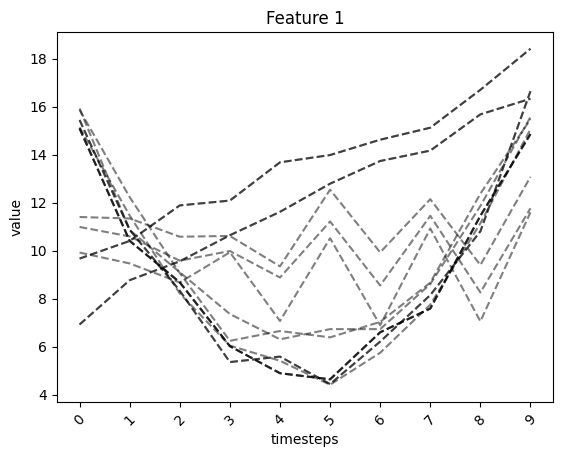
TSPlot

plot

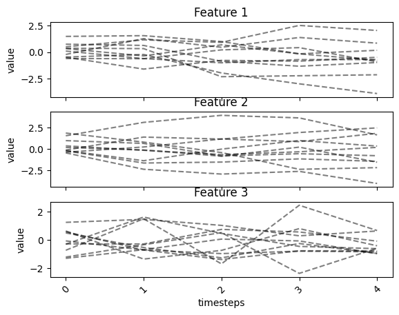
plot function is used to plot a time series plots of the different features in a time series data

fig, ax = tsplot.plot(X=X_arr)

../../../_images/tscluster_tutorial_92_0.png

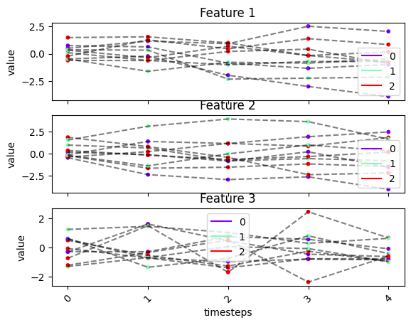
We can add label assignment to the plot

fig, ax = tsplot.plot(X=X_arr, labels=labels)

../../../_images/tscluster_tutorial_94_0.png

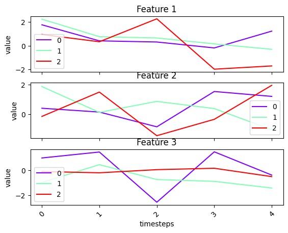
We can plot only cluster centers

fig, ax = tsplot.plot(cluster_centers=cluster_centers)

../../../_images/tscluster_tutorial_96_0.png

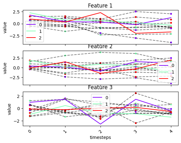
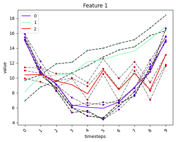
We can plot all of data X, cluster centers and label assignment in the same plot

fig, ax = tsplot.plot(X=X_arr, cluster_centers=cluster_centers, labels=labels)
# note that the cluster centers are not meaningfull since they were randomly generated

../../../_images/tscluster_tutorial_98_0.png

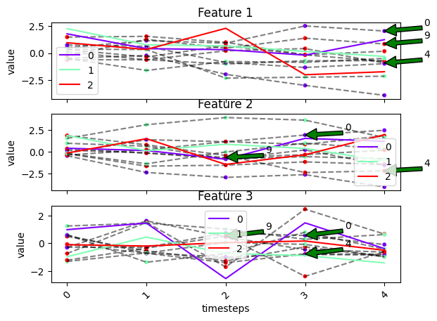
We can also annotate only specific entities by passing their index to the entity_idx parameter

fig, ax = tsplot.plot(X=X_arr, cluster_centers=cluster_centers, labels=labels, entity_idx=[0, 4, 9])

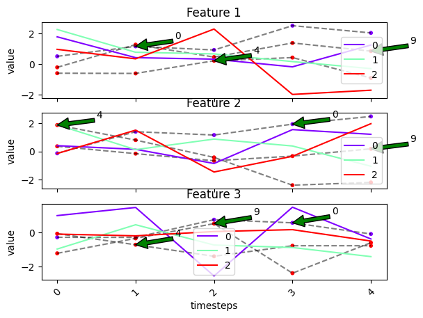
../../../_images/tscluster_tutorial_100_0.png

We can show only the entities in entity_idx by setting show_all_entities to False

fig, ax = tsplot.plot(X=X_arr, cluster_centers=cluster_centers, labels=labels, entity_idx=[0, 4, 9], show_all_entities=False)

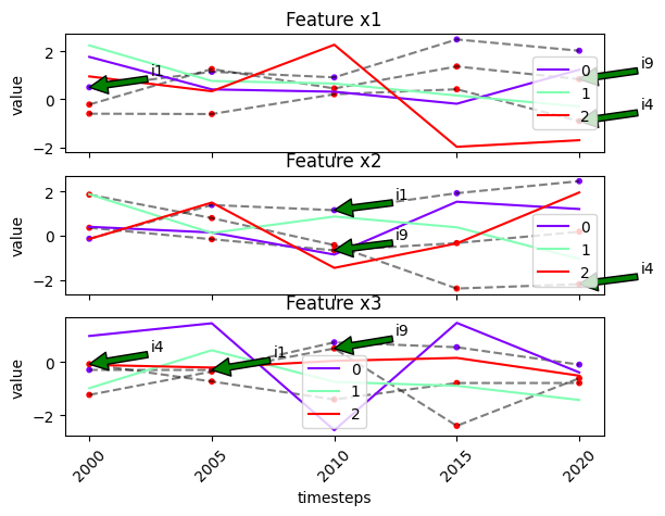
../../../_images/tscluster_tutorial_102_0.png

We can use the labels in label_dict to label the entities in entity_idx by passing label_dict

# recall our label dict
label_dict

{'T': ['2000', '2005', '2010', '2015', '2020'],
 'N': ['i1', 'i10', 'i2', 'i3', 'i4', 'i5', 'i6', 'i7', 'i8', 'i9'],
 'F': ['x1', 'x2', 'x3']}

fig, ax = tsplot.plot(
    X=X_arr,
    cluster_centers=cluster_centers,
    labels=labels,
    entity_idx=[0, 4, 9],
    show_all_entities=False,
    label_dict=label_dict
)

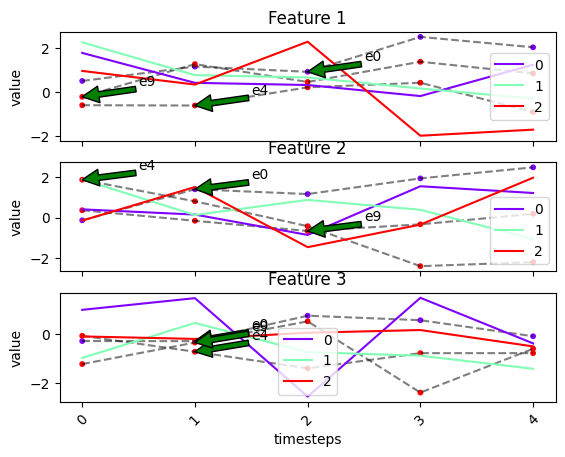
../../../_images/tscluster_tutorial_105_0.png

We can pass custom labels to the labels in entity_idx using the entities_labels parameter.

fig, ax = tsplot.plot(
    X=X_arr,
    cluster_centers=cluster_centers,
    labels=labels,
    entity_idx=[0, 4, 9],
    entities_labels=['e0', 'e4', 'e9'],
    show_all_entities=False
)

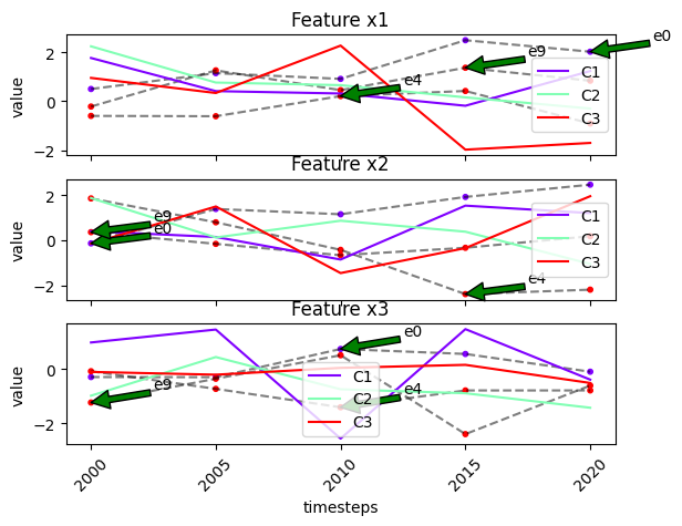
../../../_images/tscluster_tutorial_107_0.png

We can also pass custom labels for the cluster centers using the cluster_labels parameter

fig, ax = tsplot.plot(
    X=X_arr,
    cluster_centers=cluster_centers,
    labels=labels,
    entity_idx=[0, 4, 9],
    entities_labels=['e0', 'e4', 'e9'],
    show_all_entities=False,
    label_dict=label_dict,
    cluster_labels=['C1', 'C2', 'C3']
)

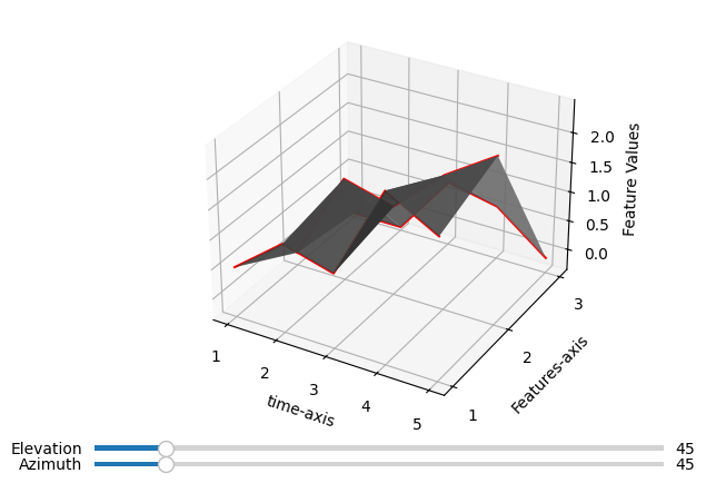
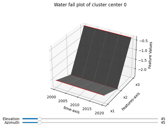
../../../_images/tscluster_tutorial_109_0.png

waterfall_plot

waterfall_plot can be used to generate a 3-D time series plot of a particular entity or cluster center.

To make the plot interactive, use a suitable matplotlib’s magic command. E.g. %matplotlib widget. See this site for more: https://matplotlib.org/stable/users/explain/figure/interactive.html

# waterfall plot of a single entity
idx = 0
fig, ax = tsplot.waterfall_plot(X_arr[:, idx, :])

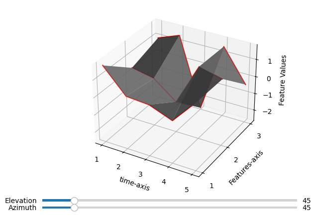
../../../_images/tscluster_tutorial_112_0.png

# waterfall plot of a single cluster center
idx = 0
fig, ax = tsplot.waterfall_plot(cluster_centers[:, idx, :])

../../../_images/tscluster_tutorial_113_0.png

Temporal Clustering Models

All temporal clustering modules implements a fit method (in which on executing, compute the cluster centers and label assignments).

We can use the cluster_centers_ and labels_ attributes to retreive the cluster centers and label assignments respectively. Here we used sklearn’s convention of using trailing underscores for attributes whose values are known only after fitting.

OptTSCluster

fixed centers, dynamic assignment

# initialize the model
opt_ts = OptTSCluster(
    n_clusters=3,
    scheme='z0c1', # fixed centers, dynamic assignment
    n_allow_assignment_change=None # number of changes to allow, None means allow as many changes as possible
    # warm_start=True # warm start with kmeans
)

model_size = opt_ts.get_model_size(X_arr)
print(f"model has {model_size[0]} variables and {model_size[1]} constraints")

Restricted license - for non-production use only - expires 2025-11-24
model has 610 variables and 950 constraints

label_dict

{'T': ['2000', '2005', '2010', '2015', '2020'],
 'N': ['i1', 'i10', 'i2', 'i3', 'i4', 'i5', 'i6', 'i7', 'i8', 'i9'],
 'F': ['x1', 'x2', 'x3']}

# fit the model
opt_ts.fit(X_arr, label_dict=label_dict); # we can optionally pass the label dict to the model during fit

Warm starting...
Done with warm start after 0.04secs

Obj val: [3.77787002]

Total time is 0.86secs

# checking the label dict
opt_ts.label_dict_

{'T': ['2000', '2005', '2010', '2015', '2020'],
 'N': ['i1', 'i10', 'i2', 'i3', 'i4', 'i5', 'i6', 'i7', 'i8', 'i9'],
 'F': ['x1', 'x2', 'x3']}

# retrieving the index of the some time labels
opt_ts.get_index_of_label(['2005', '2010'], axis='T')

[1, 2]

# retrieving the labels of the some entity indexes
opt_ts.get_label_of_index([1, 3, 0], axis='N')

['i10', 'i3', 'i1']

We can get the cluster centers as a dataframe with the labels in label_dict

cluster_centers_lst = opt_ts.get_named_cluster_centers()
cluster_centers_lst[0] # first cluster

	x1	x2	x3
2000	-2.028199	-2.377959	-0.353205
2005	-2.028199	-2.377959	-0.353205
2010	-2.028199	-2.377959	-0.353205
2015	-2.028199	-2.377959	-0.353205
2020	-2.028199	-2.377959	-0.353205

We can also get the labels as a dataframe indexed with labels in label_dict

opt_ts.get_named_labels()

	2000	2005	2010	2015	2020
i1	2	2	1	1	1
i10	2	2	0	2	0
i2	2	0	0	0	0
i3	2	2	2	1	2
i4	2	1	2	2	2
i5	1	2	0	1	2
i6	2	2	2	2	2
i7	2	0	2	1	1
i8	2	1	1	1	2
i9	2	2	2	2	1

Checking most dynamic entities

print(f"total number of cluster changes is: {opt_ts.n_changes_}")
opt_ts.get_dynamic_entities() # dynamic entities and their number of cluster changes

total number of cluster changes is: 19

(['i5', 'i7', 'i10', 'i8', 'i4', 'i3', 'i9', 'i2', 'i1'],
 [4, 3, 3, 2, 2, 2, 1, 1, 1])

# retrieve the cluster centers and labels
cc_opt_ts = opt_ts.cluster_centers_
labels_opt_ts = opt_ts.labels_
labels_opt_ts

array([[2, 2, 1, 1, 1],
       [2, 2, 0, 2, 0],
       [2, 0, 0, 0, 0],
       [2, 2, 2, 1, 2],
       [2, 1, 2, 2, 2],
       [1, 2, 0, 1, 2],
       [2, 2, 2, 2, 2],
       [2, 0, 2, 1, 1],
       [2, 1, 1, 1, 2],
       [2, 2, 2, 2, 1]])

# plot model results
fig, ax = tsplot.plot(X=X_arr, cluster_centers=cc_opt_ts, labels=labels_opt_ts, label_dict=opt_ts.label_dict_)

../../../_images/tscluster_tutorial_132_0.png

# waterfall plot of a particular cluster center
cc_idx = 0 # index of cluster center to plot
cc = broadcast_data(X_arr.shape[0], cluster_centers=cc_opt_ts)[0][:, cc_idx, :] # broadcasting the cluster center
fig, ax = tsplot.waterfall_plot(cc, label_dict=opt_ts.label_dict_)
fig.suptitle(f"Water fall plot of cluster center {cc_idx}");

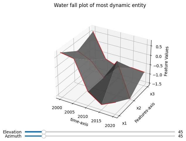
../../../_images/tscluster_tutorial_133_0.png

# waterfall plot of most dynamic entity
most_dynamic_entity_idx = np.where(opt_ts.get_named_labels().index == opt_ts.get_dynamic_entities()[0][0])[0][0]
fig, ax = tsplot.waterfall_plot(X_arr[:, most_dynamic_entity_idx, :], label_dict=opt_ts.label_dict_)
fig.suptitle("Water fall plot of most dynamic entity");

../../../_images/tscluster_tutorial_134_0.png

# scoring the model
print(f"inertia score is {inertia(X_arr, cc_opt_ts, labels_opt_ts, ord=1)}") # using l1 distance
print(f"max_dist score is {max_dist(X_arr, cc_opt_ts, labels_opt_ts, ord=1)}") # using l1 distance

inertia score is 138.84033246055895
max_dist score is 3.777870015440997

We can also set the label_dict after fitting

old_label_dict = opt_ts.label_dict_
old_label_dict

{'T': ['2000', '2005', '2010', '2015', '2020'],
 'N': ['i1', 'i10', 'i2', 'i3', 'i4', 'i5', 'i6', 'i7', 'i8', 'i9'],
 'F': ['x1', 'x2', 'x3']}

new_label_dict = {k: v for k, v in old_label_dict.items()}
new_label_dict['F'] = ['A', 'B', 'C']

opt_ts.set_label_dict(new_label_dict)

opt_ts.label_dict_

{'T': ['2000', '2005', '2010', '2015', '2020'],
 'N': ['i1', 'i10', 'i2', 'i3', 'i4', 'i5', 'i6', 'i7', 'i8', 'i9'],
 'F': ['A', 'B', 'C']}

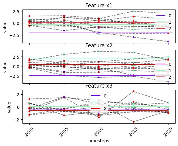
dynamic centers, fixed assignment

# loading the data
X_arr2, _ = load_data("./sythetic_data.npy")
X_arr2.shape

(10, 15, 1)

# visualizing the data
fig, ax = tsplot.plot(X=X_arr2)

../../../_images/tscluster_tutorial_142_0.png

# initialize the model
opt_ts = OptTSCluster(
    n_clusters=3,
    scheme='z1c1', # dynamic centers, dynamic assignment. Scheme needs to be a dynamic label scheme when using constrained cluster change
                   # you can also use 'z1c0' scheme here
    n_allow_assignment_change=0, # number of changes to allow, 0 means allow as no changes are allowed.
    warm_start=True # warm start with kmeans
)

# checking the size of the model
model_size = opt_ts.get_model_size(X_arr2)
print(f"model has {model_size[0]} variables and {model_size[1]} constraints")

model has 1066 variables and 1051 constraints

# fit the model
opt_ts.fit(X_arr2);

Warm starting...
Done with warm start after 0.08secs

Obj val: [1.51774178]

Total time is 0.19secs

print(f"total number of cluster changes is: {opt_ts.n_changes_}")
opt_ts.get_dynamic_entities() # indexes of dynamic entities and their number of cluster changes

total number of cluster changes is: 0

([], [])

# retrieve the cluster centers and labels
cc_opt_ts = opt_ts.cluster_centers_
labels_opt_ts = opt_ts.labels_

labels_opt_ts

array([[0, 0, 0, 0, 0, 0, 0, 0, 0, 0],
       [0, 0, 0, 0, 0, 0, 0, 0, 0, 0],
       [1, 1, 1, 1, 1, 1, 1, 1, 1, 1],
       [1, 1, 1, 1, 1, 1, 1, 1, 1, 1],
       [2, 2, 2, 2, 2, 2, 2, 2, 2, 2],
       [2, 2, 2, 2, 2, 2, 2, 2, 2, 2],
       [0, 0, 0, 0, 0, 0, 0, 0, 0, 0],
       [1, 1, 1, 1, 1, 1, 1, 1, 1, 1],
       [0, 0, 0, 0, 0, 0, 0, 0, 0, 0],
       [2, 2, 2, 2, 2, 2, 2, 2, 2, 2],
       [0, 0, 0, 0, 0, 0, 0, 0, 0, 0],
       [0, 0, 0, 0, 0, 0, 0, 0, 0, 0],
       [1, 1, 1, 1, 1, 1, 1, 1, 1, 1],
       [0, 0, 0, 0, 0, 0, 0, 0, 0, 0],
       [0, 0, 0, 0, 0, 0, 0, 0, 0, 0]])

# plot of model results
fig, ax = tsplot.plot(X=X_arr2, cluster_centers=cc_opt_ts, labels=labels_opt_ts)

../../../_images/tscluster_tutorial_149_0.png

# scoring the model
print(f"inertia score is {inertia(X_arr2, cc_opt_ts, labels_opt_ts, ord=1)}") # using l1 distance
print(f"max_dist score is {max_dist(X_arr2, cc_opt_ts, labels_opt_ts, ord=1)}") # using l1 distance

inertia score is 117.50053747638934
max_dist score is 1.5177417770731711

Bounded Changes

Creating dynamic entities

dynamic_X1 = np.concatenate([X_arr2[:3, 0, :], X_arr2[3:, 2, :]], axis=0)[:, np.newaxis, :]
dynamic_X2 = np.concatenate([X_arr2[:6, 6, :], X_arr2[6:, 4, :]], axis=0)[:, np.newaxis, :]

X_arr3 = np.concatenate([X_arr2, dynamic_X1, dynamic_X2], axis=1)
X_arr3.shape

(10, 17, 1)

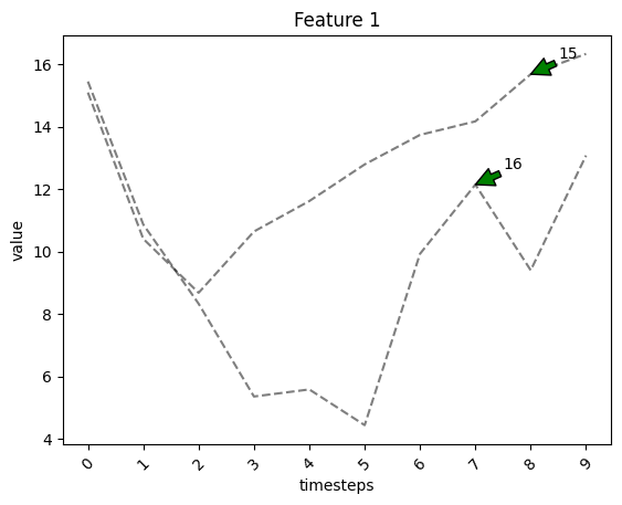
# plotting the synthetically created dynamic entities
fig, ax = tsplot.plot(X=X_arr3, entity_idx=np.arange(X_arr2.shape[1], X_arr3.shape[1]), show_all_entities=False)

../../../_images/tscluster_tutorial_155_0.png

# initialize the model
opt_ts = OptTSCluster(
    n_clusters=3,
    scheme='z1c1', # dynamic centers, dynamic assignment. Scheme needs to be a dynamic label scheme when using constrained cluster change
    n_allow_assignment_change=2, # number of changes to allow, None means allow as many changes as possible
    warm_start=True # warm start with kmeans
)

# fit the model
opt_ts.fit(X_arr3);

Warm starting...
Done with warm start after 0.05secs

Obj val: [1.51774178]

Total time is 14.4secs

# checking model's size
opt_ts.get_model_size(X_arr3)

(1204, 1191)

print(f"total number of cluster changes is: {opt_ts.n_changes_}")
opt_ts.get_dynamic_entities() # indexes of dynamic entities and their number of cluster changes

total number of cluster changes is: 2

([16, 15], [1, 1])

# retrieve the cluster centers and labels
cc_opt_ts = opt_ts.cluster_centers_
labels_opt_ts = opt_ts.labels_

# labels of dynamic entities
labels_opt_ts[opt_ts.get_dynamic_entities()[0]]

array([[2, 2, 2, 2, 2, 2, 1, 1, 1, 1],
       [2, 2, 2, 0, 0, 0, 0, 0, 0, 0]])

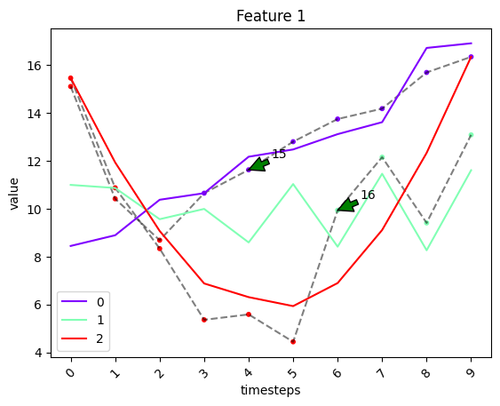
# plot of model results
fig, ax = tsplot.plot(
    X=X_arr3,
    cluster_centers=cc_opt_ts,
    labels=labels_opt_ts,
    entity_idx=opt_ts.get_dynamic_entities()[0],
    show_all_entities=False
)

../../../_images/tscluster_tutorial_161_0.png

# scoring the results
print(f"inertia score is {inertia(X_arr3, cc_opt_ts, labels_opt_ts, ord=1)}") # using l1 distance
print(f"max_dist score is {max_dist(X_arr3, cc_opt_ts, labels_opt_ts, ord=1)}") # using l1 distance

inertia score is 140.53425058177024
max_dist score is 1.5177417770731711

# checking the default label_dict (since we did not set the label dict or pass any during fit)
print(opt_ts.label_dict_)

{'T': [0, 1, 2, 3, 4, 5, 6, 7, 8, 9], 'N': [0, 1, 2, 3, 4, 5, 6, 7, 8, 9, 10, 11, 12, 13, 14, 15, 16], 'F': [0]}

TSGlobalKmeans

This module applies sklearn’s k-mean clustering to the data resulting from concatenating along the time axis.

# initialize the model
g_ts_km = TSGlobalKmeans(n_clusters=3)

# fit the model
g_ts_km.fit(X_arr3);

/usr/local/lib/python3.10/dist-packages/sklearn/cluster/_kmeans.py:870: FutureWarning: The default value of n_init will change from 10 to 'auto' in 1.4. Set the value of n_init explicitly to suppress the warning
  warnings.warn(

print(f"total number of cluster changes is: {g_ts_km.n_changes_}")
g_ts_km.get_dynamic_entities() # indexes of dynamic entities and their number of cluster changes

total number of cluster changes is: 53

([9, 16, 10, 1, 6, 8, 11, 13, 14, 0, 15, 5, 3, 2, 12, 7, 4],
 [6, 4, 4, 4, 4, 4, 4, 4, 4, 4, 2, 2, 2, 2, 1, 1, 1])

# retrieve the cluster centers and labels
cc_g_ts_km = g_ts_km.cluster_centers_
labels_g_ts_km = g_ts_km.labels_

# labels of dynamic entities
labels_g_ts_km[g_ts_km.get_dynamic_entities()[0]]

array([[0, 0, 0, 0, 2, 0, 2, 0, 2, 0],
       [1, 0, 0, 2, 2, 2, 0, 0, 0, 1],
       [1, 0, 2, 2, 2, 2, 2, 2, 0, 1],
       [1, 0, 0, 2, 2, 2, 2, 2, 0, 1],
       [1, 0, 0, 2, 2, 2, 2, 2, 0, 1],
       [1, 0, 0, 2, 2, 2, 2, 2, 0, 1],
       [1, 0, 0, 2, 2, 2, 2, 0, 0, 1],
       [1, 0, 0, 2, 2, 2, 2, 0, 0, 1],
       [1, 0, 0, 2, 2, 2, 2, 2, 0, 1],
       [1, 0, 0, 2, 2, 2, 2, 2, 0, 1],
       [1, 0, 0, 0, 0, 1, 1, 1, 1, 1],
       [0, 0, 0, 0, 0, 0, 0, 0, 2, 0],
       [2, 0, 0, 0, 0, 1, 1, 1, 1, 1],
       [2, 0, 0, 0, 0, 1, 1, 1, 1, 1],
       [0, 0, 0, 0, 1, 1, 1, 1, 1, 1],
       [0, 0, 0, 0, 1, 1, 1, 1, 1, 1],
       [0, 0, 0, 0, 0, 0, 0, 0, 0, 1]], dtype=int32)

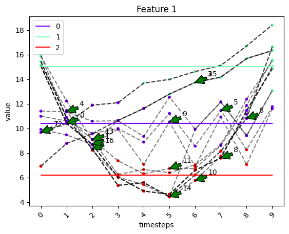
# plot of model results
fig, ax = tsplot.plot(
    X=X_arr3,
    cluster_centers=cc_g_ts_km,
    labels=labels_g_ts_km,
    entity_idx=g_ts_km.get_dynamic_entities()[0],
    show_all_entities=False
)

../../../_images/tscluster_tutorial_170_0.png

# scoring the results
print(f"inertia score is {inertia(X_arr3, cc_g_ts_km, labels_g_ts_km, ord=1)}") # using l1 distance
print(f"max_dist score is {max_dist(X_arr3, cc_g_ts_km, labels_g_ts_km, ord=1)}") # using l1 distance

inertia score is 166.82397817096967
max_dist score is 3.3717592522248783

TSKmeans

This module applies tslearn’s time series k-mean clustering to the data.

# initialize the model
ts_km = TSKmeans(n_clusters=3)

# fit the model
ts_km.fit(X_arr3);

print(f"total number of cluster changes is: {ts_km.n_changes_}")
ts_km.get_dynamic_entities() # indexes of dynamic entities and their number of cluster changes

total number of cluster changes is: 0

([], [])

# retrieve the cluster centers and labels
cc_ts_km = ts_km.cluster_centers_
labels_ts_km = ts_km.labels_

# labels of dynamic entities
labels_ts_km[ts_km.get_dynamic_entities()[0]]

array([], dtype=int64)

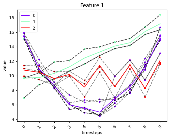
# plot of model results
fig, ax = tsplot.plot(
    X=X_arr3,
    cluster_centers=cc_ts_km,
    labels=labels_ts_km
)

../../../_images/tscluster_tutorial_178_0.png

# scoring the results
print(f"inertia score is {inertia(X_arr3, cc_ts_km, labels_ts_km, ord=1)}") # using l1 distance
print(f"max_dist score is {max_dist(X_arr3, cc_ts_km, labels_ts_km, ord=1)}") # using l1 distance

inertia score is 113.52000410204052
max_dist score is 5.437567193350128